Animating Plays in Julia with Makie.jl
Introduction
No matter what kind of project you want to tackle, you’re going to want the ability to understand what’s happening on a given play with the Big Data Bowl dataset. Easier said than done! You can go to YouTube and try to scrub through hours of film to see plays, but 1) that takes a ton of time and 2) means interfacing with the game in a meaningful way beyond manipulating a spreadsheet, which no self-respecting analytics nerd would ever do,,,
This problem has seen a lot of different approaches in previous Big Data Bowls. You can check out Nick Wan’s and Hunter Kempf’s notebooks on plotting and animating plays in Python, or Pablo Landeros' notebook on plotting and animating plays in R. But I’m not here to reinvent the wheel. I’m not some SQUARE who uses DATED PROGRAMMING LANGUAGES like some of you SHEEPLE. Besides, I’m here to push an agenda: #BringJuliaToKaggle
That’s right – we’re going to be working in Julia to produce our play visualizations. My hope is that this notebook can serve as a leaping off point for anyone who wants to do Big Data Bowl projects in Julia, and my secondary, ulterior motive is to continue to spread Julia content on Kaggle in the hopes we get dedicated support soon.
Loading in Data
To begin, let’s pull our data into our directory. I’ve already set things up with the Kaggle API to make this relatively painless. We’ll pull down not just our competition data but a few other useful visuals to help us trick out our project.
using DataFrames, CSV
function build_directory()
    run(`kaggle competitions download -c nfl-big-data-bowl-2024 --force`)
    run(`mkdir -p data`)
    run(`unzip nfl-big-data-bowl-2024.zip -d data`)
    run(`mkdir -p visuals`)
    run(`curl.exe -o visuals/bdb-logo.png https://operations.nfl.com/media/3577/big-data-bowl-transparent.png --ssl-no-revoke`)
    run(`curl.exe -o visuals/nfl-logo.png https://upload.wikimedia.org/wikipedia/en/thumb/a/a2/National_Football_League_logo.svg/745px-National_Football_League_logo.svg.png --ssl-no-revoke`)
    run(`curl.exe -o visuals/nfl-teams.csv https://raw.githubusercontent.com/nflverse/nflverse-pbp/master/teams_colors_logos.csv --ssl-no-revoke`)
    teams = CSV.read("visuals/nfl-teams.csv",DataFrame)
    for row in 1:nrow(teams)
        abbr = teams.team_abbr[row]
        run(`curl.exe -o visuals/$abbr-wordmark.png https://raw.githubusercontent.com/nflverse/nflverse-pbp/master/wordmarks/$abbr.png --ssl-no-revoke`)
    end
end
build_directory();
With our data loaded in, we can take a glimpse at what the tracking data actually looks like.
week1 = CSV.read("data/tracking_week_1.csv",DataFrame)
| Row | gameId | playId | nflId | displayName | frameId | time | jerseyNumber | club | playDirection | x | y | s | a | dis | o | dir | event |
|---|---|---|---|---|---|---|---|---|---|---|---|---|---|---|---|---|---|
| Int64 | Int64 | String7 | String31 | Int64 | String31 | String3 | String15 | String7 | Float64 | Float64 | Float64 | Float64 | Float64 | String7 | String31 | String31 | |
| 1 | 2022090800 | 56 | 35472 | Rodger Saffold | 1 | 2022-09-08 20:24:05.200000 | 76 | BUF | left | 88.37 | 27.27 | 1.62 | 1.15 | 0.16 | 231.74 | 147.9 | NA |
| 2 | 2022090800 | 56 | 35472 | Rodger Saffold | 2 | 2022-09-08 20:24:05.299999 | 76 | BUF | left | 88.47 | 27.13 | 1.67 | 0.61 | 0.17 | 230.98 | 148.53 | pass_arrived |
| 3 | 2022090800 | 56 | 35472 | Rodger Saffold | 3 | 2022-09-08 20:24:05.400000 | 76 | BUF | left | 88.56 | 27.01 | 1.57 | 0.49 | 0.15 | 230.98 | 147.05 | NA |
| 4 | 2022090800 | 56 | 35472 | Rodger Saffold | 4 | 2022-09-08 20:24:05.500000 | 76 | BUF | left | 88.64 | 26.9 | 1.44 | 0.89 | 0.14 | 232.38 | 145.42 | NA |
| 5 | 2022090800 | 56 | 35472 | Rodger Saffold | 5 | 2022-09-08 20:24:05.599999 | 76 | BUF | left | 88.72 | 26.8 | 1.29 | 1.24 | 0.13 | 233.36 | 141.95 | NA |
| 6 | 2022090800 | 56 | 35472 | Rodger Saffold | 6 | 2022-09-08 20:24:05.700000 | 76 | BUF | left | 88.8 | 26.7 | 1.15 | 1.42 | 0.12 | 234.48 | 139.41 | pass_outcome_caught |
| 7 | 2022090800 | 56 | 35472 | Rodger Saffold | 7 | 2022-09-08 20:24:05.799999 | 76 | BUF | left | 88.87 | 26.64 | 0.93 | 1.69 | 0.09 | 235.77 | 134.32 | NA |
| 8 | 2022090800 | 56 | 35472 | Rodger Saffold | 8 | 2022-09-08 20:24:05.900000 | 76 | BUF | left | 88.91 | 26.59 | 0.68 | 1.74 | 0.07 | 240 | 131.01 | NA |
| 9 | 2022090800 | 56 | 35472 | Rodger Saffold | 9 | 2022-09-08 20:24:06.000000 | 76 | BUF | left | 88.94 | 26.57 | 0.42 | 1.74 | 0.04 | 243.56 | 122.29 | NA |
| 10 | 2022090800 | 56 | 35472 | Rodger Saffold | 10 | 2022-09-08 20:24:06.099999 | 76 | BUF | left | 88.95 | 26.58 | 0.14 | 1.83 | 0.01 | 246.07 | 85.87 | NA |
| 11 | 2022090800 | 56 | 35472 | Rodger Saffold | 11 | 2022-09-08 20:24:06.200000 | 76 | BUF | left | 88.92 | 26.6 | 0.26 | 1.9 | 0.03 | 252.65 | 326.63 | NA |
| 12 | 2022090800 | 56 | 35472 | Rodger Saffold | 12 | 2022-09-08 20:24:06.299999 | 76 | BUF | left | 88.9 | 26.63 | 0.51 | 2.45 | 0.04 | 257.66 | 315.55 | NA |
| 13 | 2022090800 | 56 | 35472 | Rodger Saffold | 13 | 2022-09-08 20:24:06.400000 | 76 | BUF | left | 88.84 | 26.68 | 0.81 | 2.03 | 0.08 | 262.09 | 311.72 | NA |
| ⋮ | ⋮ | ⋮ | ⋮ | ⋮ | ⋮ | ⋮ | ⋮ | ⋮ | ⋮ | ⋮ | ⋮ | ⋮ | ⋮ | ⋮ | ⋮ | ⋮ | ⋮ |
| 1407428 | 2022091200 | 3826 | NA | football | 42 | 2022-09-12 23:05:57.099999 | NA | football | left | 57.13 | 8.44 | 2.17 | 3.63 | 0.29 | NA | NA | NA |
| 1407429 | 2022091200 | 3826 | NA | football | 43 | 2022-09-12 23:05:57.200000 | NA | football | left | 56.99 | 8.66 | 2.01 | 2.68 | 0.26 | NA | NA | NA |
| 1407430 | 2022091200 | 3826 | NA | football | 44 | 2022-09-12 23:05:57.299999 | NA | football | left | 56.85 | 8.87 | 1.97 | 1.7 | 0.25 | NA | NA | NA |
| 1407431 | 2022091200 | 3826 | NA | football | 45 | 2022-09-12 23:05:57.400000 | NA | football | left | 56.76 | 9.04 | 1.83 | 1.14 | 0.19 | NA | NA | NA |
| 1407432 | 2022091200 | 3826 | NA | football | 46 | 2022-09-12 23:05:57.500000 | NA | football | left | 56.63 | 9.28 | 2.15 | 0.33 | 0.27 | NA | NA | NA |
| 1407433 | 2022091200 | 3826 | NA | football | 47 | 2022-09-12 23:05:57.599999 | NA | football | left | 56.52 | 9.5 | 2.34 | 1.12 | 0.24 | NA | NA | NA |
| 1407434 | 2022091200 | 3826 | NA | football | 48 | 2022-09-12 23:05:57.700000 | NA | football | left | 56.4 | 9.72 | 2.53 | 1.23 | 0.26 | NA | NA | NA |
| 1407435 | 2022091200 | 3826 | NA | football | 49 | 2022-09-12 23:05:57.799999 | NA | football | left | 56.22 | 9.89 | 2.56 | 1.25 | 0.25 | NA | NA | tackle |
| 1407436 | 2022091200 | 3826 | NA | football | 50 | 2022-09-12 23:05:57.900000 | NA | football | left | 56.06 | 10.08 | 2.5 | 1.14 | 0.24 | NA | NA | NA |
| 1407437 | 2022091200 | 3826 | NA | football | 51 | 2022-09-12 23:05:58.000000 | NA | football | left | 55.89 | 10.27 | 2.38 | 1.7 | 0.25 | NA | NA | NA |
| 1407438 | 2022091200 | 3826 | NA | football | 52 | 2022-09-12 23:05:58.099999 | NA | football | left | 55.73 | 10.44 | 2.07 | 2.83 | 0.24 | NA | NA | NA |
| 1407439 | 2022091200 | 3826 | NA | football | 53 | 2022-09-12 23:05:58.200000 | NA | football | left | 55.57 | 10.57 | 1.86 | 3.0 | 0.2 | NA | NA | NA |
The available tracking data is split up into several different components:
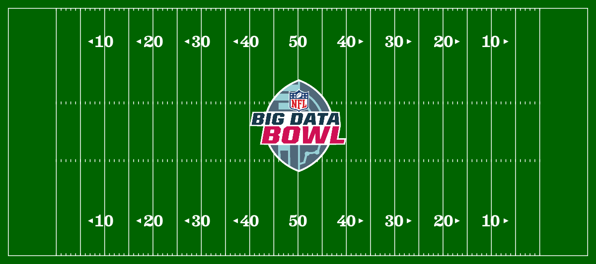
gameId– A unique identifier assigned to each gameplayId– A unique identifier assigned to each playframeId– The frame of the play For each unique combination ofgameId,playId, andframeId, we have thexandycoordinates of each player (identified with any ofnflId,displayName, orjerseyNumber) as well as the football. Thexandycoordinates are laid out as demonstrated in this graphic, helpfully provided by the organizers by the Big Data Bowl:
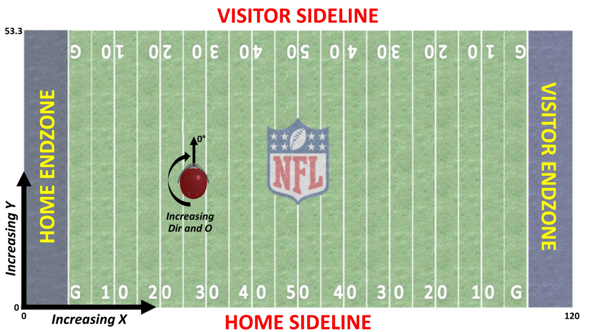
We can use this plot as a guide to generating our own graphic in Julia.
Groundskeeping
Our first step is to build the field on which plays will take place. We will use Makie.jl as the plotting library for our visuals – it’s the most flexible library for plotting in Julia, and should allow us to manipulate and animate the play we want. Specifically, we’ll import CairoMakie, which will allow us to render high quality graphics using the Cairo backend.
What’s the first step to building a football field? Laying down the grass, of course – we’ll make a green background that fits the coordinate system described in the graphic above. Note that this can take a while to render initially – after compiling everything, it should run much faster thanks to Julia magic 🪄.
using CairoMakie
function base_figure()
    f = Figure(backgroundcolor = :darkgreen, resolution = (1200,533))
    ax = Axis(f[1,1], limits = (0,120,0,53.3), backgroundcolor = :darkgreen)
    hidedecorations!(ax)
    hidespines!(ax)
    return f, ax
end
f, ax = base_figure()
f

Next, we’ll be good groundskeepers and paint the lines.
using GeometryBasics
f, = base_figure()
poly!(
    Rect(0,0,120,53.3),
    strokecolor = :white,
    strokewidth = 3,
    color = :darkgreen
)
f

This football field could use some lines. Let’s bust out our tape measure and start marking out the field!
vlines!(
    10:5:110,
    color = :white
)
f

That’s looking good, but how will we know where the spot the ball? After all, not like there’s a chip in the football or anything,,, this field clearly needs some line numbers.
text!(
    18:10:98,
    repeat([5],9);
    text = string.([10:10:50; 40:-10:10]),
    font="C:/Users/edwar/Documents/GitHub/bdb24/visuals/besley_heavy.otf",
    fontsize=30,
    color=:white
    )
text!(
    18:10:98,
    repeat([43.5],9);
    text = string.([10:10:50; 40:-10:10]),
    font="C:/Users/edwar/Documents/GitHub/bdb24/visuals/besley_heavy.otf",
    fontsize=30,
    color=:white
)
f
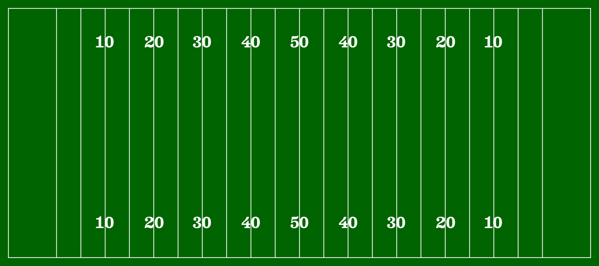
Great! Now, we need some arrows, just to make sure everyone knows which way to run the ball. We can use some ASCII text art to quickly throw some on our plot.
text!(
    16.5:10:46.5,
    repeat([6.5],4);
    text = repeat(["◂"],4),
    fontsize=20,
    color=:white
)
text!(
    16.5:10:46.5,
    repeat([45],4);
    text = repeat(["◂"],4),
    fontsize=20,
    color=:white
)
text!(
    72.5:10:102.5,
    repeat([6.5],4);
    text = repeat(["▸"],4),
    fontsize=20,
    color=:white
)
text!(
    72.5:10:102.5,
    repeat([45],4);
    text = repeat(["▸"],4),
    fontsize=20,
    color=:white
)
f
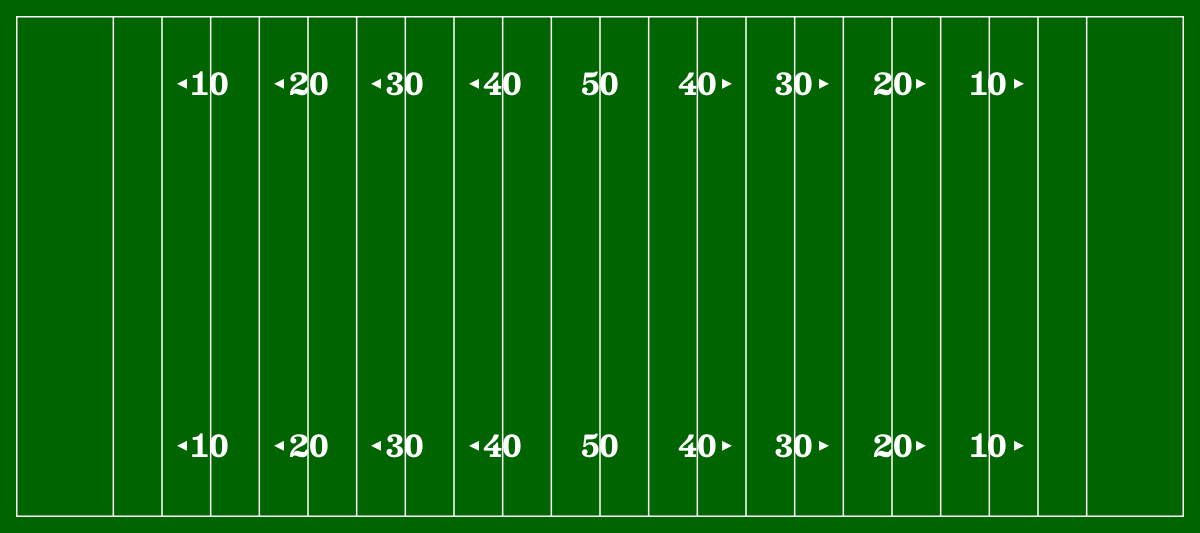
We’re cooking so far! But how will our kickers know where to kick from? This field is in need of hash marks.
vlines!(
    10:1:110;
    ymin = 0 / 53.3, # these are a percentage of the plotting window, not absolute coordinates
    ymax = 0.6 / 53.3,
    color = :white
)
vlines!(
    10:1:110;
    ymin = 52.7 / 53.3,
    ymax = 53.3 / 53.3,
    color = :white
)
vlines!(
    10:1:110;
    ymin = 20.2 / 53.3,
    ymax = 20.8 / 53.3,
    color = :white
)
vlines!(
    10:1:110;
    ymin = 33.2 / 53.3,
    ymax = 32.6 / 53.3,
    color = :white
)
f

Now that’s a proper, self-respecting football field! But we’re still missing one thing… that’s right, an enormous, obnoxious logo smack dab in the center of the field. Fortunately, adding it is a cinch with Makie.
using FileIO
img = load("visuals/bdb-logo.png")
image!(
    [50,70],[18,38],rotr90(img)
)
f
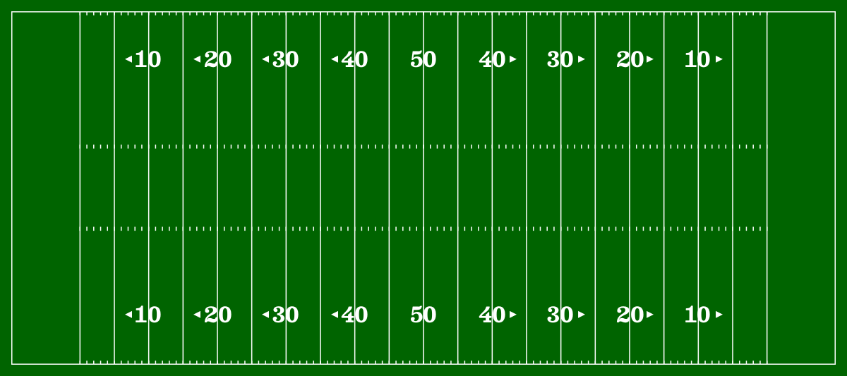
Our field looks ready to go! We can wrap everything in a function for convenience’s sake and just call on that whenever we need to plot on top of a field.
f, = base_figure()
function plot_field(logo=false)
    # background
    # remove plot decorations
    # exterior lines
    poly!(
        Rect(0,0,120,53.3),
        strokecolor = :white,
        strokewidth = 3,
        color = :darkgreen
    )
    # interior lines
    vlines!(
        10:5:110,
        color = :white
    )
    # hash marks
    vlines!(
        10:1:110;
        ymin = 0 / 53.3, # these are a percentage of the plotting window, not absolute coordinates
        ymax = 0.6 / 53.3,
        color = :white
    )
    vlines!(
        10:1:110;
        ymin = 52.7 / 53.3,
        ymax = 53.3 / 53.3,
        color = :white
    )
    vlines!(
        10:1:110;
        ymin = 20.2 / 53.3,
        ymax = 20.8 / 53.3,
        color = :white
    )
    vlines!(
        10:1:110;
        ymin = 33.2 / 53.3,
        ymax = 32.6 / 53.3,
        color = :white
    )
    # field numbers
    text!(
        18:10:98,
        repeat([5],9);
        text = string.([10:10:50; 40:-10:10]),
        font="C:/Users/edwar/Documents/GitHub/bdb24/visuals/besley_heavy.otf",
        fontsize=30,
        color=:white
        )
    text!(
        18:10:98,
        repeat([43.5],9);
        text = string.([10:10:50; 40:-10:10]),
        font="C:/Users/edwar/Documents/GitHub/bdb24/visuals/besley_heavy.otf",
        fontsize=30,
        color=:white
    )
    # field arrows
    text!(
        16.5:10:46.5,
        repeat([6.5],4);
        text = repeat(["◂"],4),
        fontsize=20,
        color=:white
    )
    text!(
        16.5:10:46.5,
        repeat([45],4);
        text = repeat(["◂"],4),
        fontsize=20,
        color=:white
    )
    text!(
        72.5:10:102.5,
        repeat([6.5],4);
        text = repeat(["▸"],4),
        fontsize=20,
        color=:white
    )
    text!(
        72.5:10:102.5,
        repeat([45],4);
        text = repeat(["▸"],4),
        fontsize=20,
        color=:white
    )
    if logo
        img = load("visuals/bdb-logo.png")
        image!(
            [50,70],[18,38],rotr90(img)
        )
    end
    return f, ax
end
plot_field()
f
Play Action
Our next step is to plot the players on the field for a given frame. For simplicity’s sake, let’s start out just plotting a random frame from a random play in week 1.
frame = week1[(week1.gameId .== 2022091100) .& (week1.playId .== 1608) .& (week1.frameId .== 1),:]
| Row | gameId | playId | nflId | displayName | frameId | time | jerseyNumber | club | playDirection | x | y | s | a | dis | o | dir | event |
|---|---|---|---|---|---|---|---|---|---|---|---|---|---|---|---|---|---|
| Int64 | Int64 | String7 | String31 | Int64 | String31 | String3 | String15 | String7 | Float64 | Float64 | Float64 | Float64 | Float64 | String7 | String31 | String31 | |
| 1 | 2022091100 | 1608 | 38607 | Demario Davis | 1 | 2022-09-11 14:14:42.400000 | 56 | NO | left | 56.66 | 25.97 | 0.0 | 0.0 | 0.0 | 80.84 | 240.31 | NA |
| 2 | 2022091100 | 1608 | 39975 | Cordarrelle Patterson | 1 | 2022-09-11 14:14:42.400000 | 84 | ATL | left | 68.78 | 23.69 | 0.0 | 0.0 | 0.0 | 259.23 | 300.66 | NA |
| 3 | 2022091100 | 1608 | 40017 | Tyrann Mathieu | 1 | 2022-09-11 14:14:42.400000 | 32 | NO | left | 52.97 | 17.53 | 0.0 | 0.0 | 0.02 | 67.67 | 250.77 | NA |
| 4 | 2022091100 | 1608 | 41232 | Jake Matthews | 1 | 2022-09-11 14:14:42.400000 | 70 | ATL | left | 62.45 | 20.62 | 0.0 | 0.0 | 0.0 | 272.22 | 196.4 | NA |
| 5 | 2022091100 | 1608 | 41257 | Bradley Roby | 1 | 2022-09-11 14:14:42.400000 | 21 | NO | left | 52.82 | 34.89 | 0.11 | 0.45 | 0.01 | 26.97 | 53.25 | NA |
| 6 | 2022091100 | 1608 | 42345 | Marcus Mariota | 1 | 2022-09-11 14:14:42.400000 | 1 | ATL | left | 62.8 | 23.72 | 0.0 | 0.0 | 0.0 | 256.19 | 167.66 | NA |
| 7 | 2022091100 | 1608 | 42553 | Christian Ringo | 1 | 2022-09-11 14:14:42.400000 | 57 | NO | left | 60.5 | 24.63 | 0.0 | 0.0 | 0.0 | 87.24 | 96.17 | NA |
| 8 | 2022091100 | 1608 | 44823 | Marshon Lattimore | 1 | 2022-09-11 14:14:42.400000 | 23 | NO | left | 60.29 | 14.52 | 0.0 | 0.0 | 0.0 | 359.05 | 14.58 | NA |
| 9 | 2022091100 | 1608 | 44851 | Marcus Maye | 1 | 2022-09-11 14:14:42.400000 | 6 | NO | left | 46.55 | 26.75 | 0.67 | 0.9 | 0.07 | 88.19 | 246.27 | NA |
| 10 | 2022091100 | 1608 | 44862 | Justin Evans | 1 | 2022-09-11 14:14:42.400000 | 30 | NO | left | 59.35 | 30.64 | 0.0 | 0.0 | 0.0 | 107.49 | 281.42 | NA |
| 11 | 2022091100 | 1608 | 45550 | Elijah Wilkinson | 1 | 2022-09-11 14:14:42.400000 | 68 | ATL | left | 62.39 | 22.4 | 0.0 | 0.0 | 0.0 | 241.48 | 51.29 | NA |
| 12 | 2022091100 | 1608 | 46083 | Marcus Davenport | 1 | 2022-09-11 14:14:42.400000 | 92 | NO | left | 60.41 | 18.29 | 0.0 | 0.0 | 0.0 | 52.63 | 326.14 | NA |
| 13 | 2022091100 | 1608 | 46197 | Kentavius Street | 1 | 2022-09-11 14:14:42.400000 | 91 | NO | left | 60.44 | 21.83 | 0.0 | 0.0 | 0.0 | 81.96 | 118.2 | NA |
| 14 | 2022091100 | 1608 | 47797 | Chris Lindstrom | 1 | 2022-09-11 14:14:42.400000 | 63 | ATL | left | 62.09 | 25.1 | 0.0 | 0.0 | 0.0 | 250.06 | 27.22 | NA |
| 15 | 2022091100 | 1608 | 47814 | Kaleb McGary | 1 | 2022-09-11 14:14:42.400000 | 76 | ATL | left | 62.29 | 26.68 | 0.0 | 0.0 | 0.0 | 262.33 | 295.83 | NA |
| 16 | 2022091100 | 1608 | 48723 | Parker Hesse | 1 | 2022-09-11 14:14:42.400000 | 46 | ATL | left | 62.81 | 29.37 | 0.0 | 0.0 | 0.0 | 250.23 | 209.71 | NA |
| 17 | 2022091100 | 1608 | 52489 | Bryan Edwards | 1 | 2022-09-11 14:14:42.400000 | 89 | ATL | left | 63.57 | 33.01 | 0.0 | 0.0 | 0.0 | 278.91 | 178.09 | NA |
| 18 | 2022091100 | 1608 | 53433 | Kyle Pitts | 1 | 2022-09-11 14:14:42.400000 | 8 | ATL | left | 62.56 | 27.83 | 0.0 | 0.0 | 0.0 | 221.39 | 299.25 | NA |
| 19 | 2022091100 | 1608 | 53457 | Payton Turner | 1 | 2022-09-11 14:14:42.400000 | 98 | NO | left | 60.41 | 27.64 | 0.0 | 0.0 | 0.0 | 101.17 | 260.18 | NA |
| 20 | 2022091100 | 1608 | 53489 | Pete Werner | 1 | 2022-09-11 14:14:42.400000 | 20 | NO | left | 56.45 | 22.09 | 0.0 | 0.0 | 0.0 | 94.74 | 203.69 | NA |
| 21 | 2022091100 | 1608 | 53543 | Drew Dalman | 1 | 2022-09-11 14:14:42.400000 | 67 | ATL | left | 61.79 | 23.64 | 0.0 | 0.0 | 0.0 | 264.7 | 305.59 | NA |
| 22 | 2022091100 | 1608 | 54473 | Drake London | 1 | 2022-09-11 14:14:42.400000 | 5 | ATL | left | 62.43 | 14.69 | 0.0 | 0.0 | 0.0 | 297.2 | 104.64 | NA |
| 23 | 2022091100 | 1608 | NA | football | 1 | 2022-09-11 14:14:42.400000 | NA | football | left | 61.55 | 23.73 | 0.0 | 0.0 | 0.0 | NA | NA | NA |
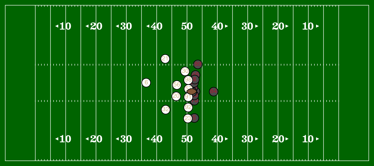
We can represent all of the players on the field as little dots (as is the convention in showing this kind of tracking data). We can treat this as a scatterplot in Makie.
f, = base_figure()
plot_field()
scatter!(frame.x, frame.y)
f
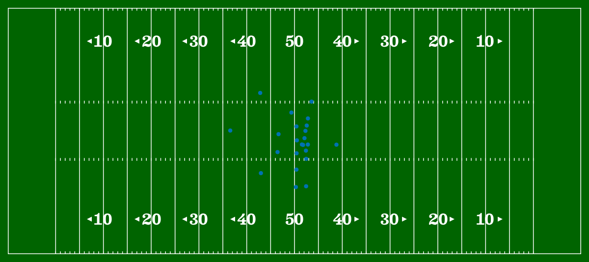
This is a good start, but this really doesn’t show us much about the frame in question. Who belongs to which team? Who is each player? Where’s the ball???
We can identify who belongs to each team by coloring them uniquely. This can be a little tricky – some teams share primary colors, some teams share secondary colors – picking which color to use for each team is tricky! I’ve gone through and tried to pick out a dark and light variant of a color from each team’s color scheme, as well as a color for text that shows up well on both the light and dark colors. You can check out my work on this stored as a .csv here . We’ll follow this set of rules for determining the colors to be used:
- If
clubis the football, color the dot brown (already covered in the .csv) - If
clubis the home team, color the dot the light-variant of the team’s color. - If
clubis the road team, color the dot the dark-variant of the team’s color.
team_colors = CSV.read(download("https://gist.githubusercontent.com/john-b-edwards/7197daa7128088f2cb5bddef4e09bfa7/raw/8af4fb83609104fa14950cde5cc31d4d95a247b9/nfl_colors.csv"), DataFrame)
games = CSV.read("data/games.csv",DataFrame)
home_away = games[:,[:gameId, :homeTeamAbbr]]
frame = innerjoin(frame,team_colors,on = :club => :team)
frame = innerjoin(frame,home_away,on = :gameId)
frame.color = ifelse.(frame.homeTeamAbbr .== frame.club, frame.dark, frame.light)
frame
| Row | gameId | playId | nflId | displayName | frameId | time | jerseyNumber | club | playDirection | x | y | s | a | dis | o | dir | event | dark | light | text | homeTeamAbbr | color |
|---|---|---|---|---|---|---|---|---|---|---|---|---|---|---|---|---|---|---|---|---|---|---|
| Int64 | Int64 | String7 | String31 | Int64 | String31 | String3 | String15 | String7 | Float64 | Float64 | Float64 | Float64 | Float64 | String7 | String31 | String31 | String7 | String7 | String7 | String3 | String7 | |
| 1 | 2022091100 | 1608 | 39975 | Cordarrelle Patterson | 1 | 2022-09-11 14:14:42.400000 | 84 | ATL | left | 68.78 | 23.69 | 0.0 | 0.0 | 0.0 | 259.23 | 300.66 | NA | #4b4b4b | #A5ACAF | #A71930 | ATL | #4b4b4b |
| 2 | 2022091100 | 1608 | 41232 | Jake Matthews | 1 | 2022-09-11 14:14:42.400000 | 70 | ATL | left | 62.45 | 20.62 | 0.0 | 0.0 | 0.0 | 272.22 | 196.4 | NA | #4b4b4b | #A5ACAF | #A71930 | ATL | #4b4b4b |
| 3 | 2022091100 | 1608 | 42345 | Marcus Mariota | 1 | 2022-09-11 14:14:42.400000 | 1 | ATL | left | 62.8 | 23.72 | 0.0 | 0.0 | 0.0 | 256.19 | 167.66 | NA | #4b4b4b | #A5ACAF | #A71930 | ATL | #4b4b4b |
| 4 | 2022091100 | 1608 | 45550 | Elijah Wilkinson | 1 | 2022-09-11 14:14:42.400000 | 68 | ATL | left | 62.39 | 22.4 | 0.0 | 0.0 | 0.0 | 241.48 | 51.29 | NA | #4b4b4b | #A5ACAF | #A71930 | ATL | #4b4b4b |
| 5 | 2022091100 | 1608 | 47797 | Chris Lindstrom | 1 | 2022-09-11 14:14:42.400000 | 63 | ATL | left | 62.09 | 25.1 | 0.0 | 0.0 | 0.0 | 250.06 | 27.22 | NA | #4b4b4b | #A5ACAF | #A71930 | ATL | #4b4b4b |
| 6 | 2022091100 | 1608 | 47814 | Kaleb McGary | 1 | 2022-09-11 14:14:42.400000 | 76 | ATL | left | 62.29 | 26.68 | 0.0 | 0.0 | 0.0 | 262.33 | 295.83 | NA | #4b4b4b | #A5ACAF | #A71930 | ATL | #4b4b4b |
| 7 | 2022091100 | 1608 | 48723 | Parker Hesse | 1 | 2022-09-11 14:14:42.400000 | 46 | ATL | left | 62.81 | 29.37 | 0.0 | 0.0 | 0.0 | 250.23 | 209.71 | NA | #4b4b4b | #A5ACAF | #A71930 | ATL | #4b4b4b |
| 8 | 2022091100 | 1608 | 52489 | Bryan Edwards | 1 | 2022-09-11 14:14:42.400000 | 89 | ATL | left | 63.57 | 33.01 | 0.0 | 0.0 | 0.0 | 278.91 | 178.09 | NA | #4b4b4b | #A5ACAF | #A71930 | ATL | #4b4b4b |
| 9 | 2022091100 | 1608 | 53433 | Kyle Pitts | 1 | 2022-09-11 14:14:42.400000 | 8 | ATL | left | 62.56 | 27.83 | 0.0 | 0.0 | 0.0 | 221.39 | 299.25 | NA | #4b4b4b | #A5ACAF | #A71930 | ATL | #4b4b4b |
| 10 | 2022091100 | 1608 | 53543 | Drew Dalman | 1 | 2022-09-11 14:14:42.400000 | 67 | ATL | left | 61.79 | 23.64 | 0.0 | 0.0 | 0.0 | 264.7 | 305.59 | NA | #4b4b4b | #A5ACAF | #A71930 | ATL | #4b4b4b |
| 11 | 2022091100 | 1608 | 54473 | Drake London | 1 | 2022-09-11 14:14:42.400000 | 5 | ATL | left | 62.43 | 14.69 | 0.0 | 0.0 | 0.0 | 297.2 | 104.64 | NA | #4b4b4b | #A5ACAF | #A71930 | ATL | #4b4b4b |
| 12 | 2022091100 | 1608 | 38607 | Demario Davis | 1 | 2022-09-11 14:14:42.400000 | 56 | NO | left | 56.66 | 25.97 | 0.0 | 0.0 | 0.0 | 80.84 | 240.31 | NA | #101820 | #FFFFFF | #D3BC8D | ATL | #FFFFFF |
| 13 | 2022091100 | 1608 | 40017 | Tyrann Mathieu | 1 | 2022-09-11 14:14:42.400000 | 32 | NO | left | 52.97 | 17.53 | 0.0 | 0.0 | 0.02 | 67.67 | 250.77 | NA | #101820 | #FFFFFF | #D3BC8D | ATL | #FFFFFF |
| 14 | 2022091100 | 1608 | 41257 | Bradley Roby | 1 | 2022-09-11 14:14:42.400000 | 21 | NO | left | 52.82 | 34.89 | 0.11 | 0.45 | 0.01 | 26.97 | 53.25 | NA | #101820 | #FFFFFF | #D3BC8D | ATL | #FFFFFF |
| 15 | 2022091100 | 1608 | 42553 | Christian Ringo | 1 | 2022-09-11 14:14:42.400000 | 57 | NO | left | 60.5 | 24.63 | 0.0 | 0.0 | 0.0 | 87.24 | 96.17 | NA | #101820 | #FFFFFF | #D3BC8D | ATL | #FFFFFF |
| 16 | 2022091100 | 1608 | 44823 | Marshon Lattimore | 1 | 2022-09-11 14:14:42.400000 | 23 | NO | left | 60.29 | 14.52 | 0.0 | 0.0 | 0.0 | 359.05 | 14.58 | NA | #101820 | #FFFFFF | #D3BC8D | ATL | #FFFFFF |
| 17 | 2022091100 | 1608 | 44851 | Marcus Maye | 1 | 2022-09-11 14:14:42.400000 | 6 | NO | left | 46.55 | 26.75 | 0.67 | 0.9 | 0.07 | 88.19 | 246.27 | NA | #101820 | #FFFFFF | #D3BC8D | ATL | #FFFFFF |
| 18 | 2022091100 | 1608 | 44862 | Justin Evans | 1 | 2022-09-11 14:14:42.400000 | 30 | NO | left | 59.35 | 30.64 | 0.0 | 0.0 | 0.0 | 107.49 | 281.42 | NA | #101820 | #FFFFFF | #D3BC8D | ATL | #FFFFFF |
| 19 | 2022091100 | 1608 | 46083 | Marcus Davenport | 1 | 2022-09-11 14:14:42.400000 | 92 | NO | left | 60.41 | 18.29 | 0.0 | 0.0 | 0.0 | 52.63 | 326.14 | NA | #101820 | #FFFFFF | #D3BC8D | ATL | #FFFFFF |
| 20 | 2022091100 | 1608 | 46197 | Kentavius Street | 1 | 2022-09-11 14:14:42.400000 | 91 | NO | left | 60.44 | 21.83 | 0.0 | 0.0 | 0.0 | 81.96 | 118.2 | NA | #101820 | #FFFFFF | #D3BC8D | ATL | #FFFFFF |
| 21 | 2022091100 | 1608 | 53457 | Payton Turner | 1 | 2022-09-11 14:14:42.400000 | 98 | NO | left | 60.41 | 27.64 | 0.0 | 0.0 | 0.0 | 101.17 | 260.18 | NA | #101820 | #FFFFFF | #D3BC8D | ATL | #FFFFFF |
| 22 | 2022091100 | 1608 | 53489 | Pete Werner | 1 | 2022-09-11 14:14:42.400000 | 20 | NO | left | 56.45 | 22.09 | 0.0 | 0.0 | 0.0 | 94.74 | 203.69 | NA | #101820 | #FFFFFF | #D3BC8D | ATL | #FFFFFF |
| 23 | 2022091100 | 1608 | NA | football | 1 | 2022-09-11 14:14:42.400000 | NA | football | left | 61.55 | 23.73 | 0.0 | 0.0 | 0.0 | NA | NA | NA | #825736 | #825736 | #825736 | ATL | #825736 |
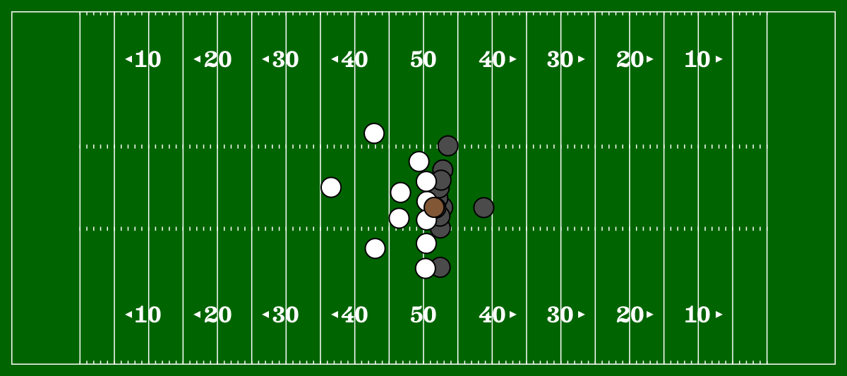
Now that we’ve applied our color rules, we can scatter out dots on the field, and tag them as the appropriate color.
f, = base_figure()
plot_field()
scatter!(
    frame.x,
    frame.y;
    color = String.(frame.color),
    markersize = 40,
    strokewidth=2
)
f
To better identify the players on the field, we can also overlay their uniform numbers on top of the play.
text!(
    frame.x[frame.club .!= "football"],
    frame.y[frame.club .!= "football"];
    text = String.(frame.jerseyNumber[frame.club .!= "football"]),
    font = "Helvetica",
    fontstyle = :bold,
    fontsize=20,
    color=String.(frame.text[frame.club .!= "football"]),
    align = (:center, :center)
)
f

Hrm, that’s problematic – the text representing all the players overlaps significantly, causing a big mess in the middle of the scene.
It’s slightly less efficient, but let’s re-work our code to iterately place each player’s dot and then text, to fix this overlapping text issue. This is slightly less efficient from a computational lens, but this is also Julia, where everything runs lightning fast, so who the #$@! cares???
f, = base_figure()
plot_field()
for n in 1:nrow(frame)
    scatter!(
        frame.x[n],
        frame.y[n];
        color = String.(frame.color[n]),
        markersize = 40,
        strokewidth=2
    )
    if frame.club[n] != "football"
        text!(
            frame.x[n],
            frame.y[n];
            text = String.(frame.jerseyNumber[n]),
            font = "Helvetica",
            fontstyle = :bold,
            fontsize=20,
            color=String.(frame.text[n]),
            align = (:center, :center)
        )
    end
end
f

Visually, that looks much better – we’re going for a “player tokens” look, and this captures that vibe quite well.
Speaking of tokens – that football looks pretty whack. Who ever heard of a round football? This isn’t Europe, we call that soccer in these here parts. 🇺🇸
function football()
    # from https://upload.wikimedia.org/wikipedia/commons/2/2d/American_football_icon_simple_flat.svg
    football_string = "M260.23 242.48C470.17 49.91 703.98 47.53 770.09 50.38c54.62 2.3575 100.81 8.0024 121.59 12.397 34.724 7.3432 25.195 7.327 46.702 33.008 21.507 25.681 34.249 26.987 35.022 68.388.63801 34.21 5.9807 206.33-60.35 357.28-66.33 150.96-113.03 188.58-173.28 243.85-60.25 55.26-197.57 142.87-350.57 174.11-79.27 16.19-298.03 7.65-312.03-10.34-5.637-8.26-14.161-17.48-20.932-22.5-15.188-16.56-25.367-51.22-26.948-79.87-1.581-28.65-13.148-189.89 60.548-346.12 73.692-156.24 170.39-238.1 170.39-238.1z"
    symbol = BezierPath(football_string, fit = true)
    return(symbol)
end

f, = base_figure()
plot_field()

for n in 1:nrow(frame)
    if frame.club[n] != "football"
    scatter!(
        frame.x[n],
        frame.y[n];
        color = String.(frame.color[n]),
        markersize = 40,
        strokewidth=2
    )
    text!(
        frame.x[n],
        frame.y[n];
        text = String.(frame.jerseyNumber[n]),
        font = "Helvetica",
        fontstyle = :bold,
        fontsize=20,
        color=String.(frame.text[n]),
        align = (:center, :center)
    )
    else
        scatter!(
            frame.x[n],
            frame.y[n];
            marker = football(),
            color = String.(frame.color[n]),
            rotations = pi / 4,
            markersize = 25,
            strokewidth=2
        )
    end
end
f
Looking great so far! We can wrap this in a function to make plotting the players a little easier.
function plot_players(frame)
    for n in 1:nrow(frame)
        if frame.club[n] != "football"
        scatter!(
            frame.x[n],
            frame.y[n];
            color = String.(frame.color[n]),
            markersize = 40,
            strokewidth=2
        )
        text!(
            frame.x[n],
            frame.y[n];
            text = String.(frame.jerseyNumber[n]),
            font = "Helvetica",
            fontstyle = :bold,
            fontsize=20,
            color=String.(frame.text[n]),
            align = (:center, :center)
        )
        else
            scatter!(
                frame.x[n],
                frame.y[n];
                marker = football(),
                color = String.(frame.color[n]),
                rotations = pi / 4,
                markersize = 25,
                strokewidth=2
            )
        end
    end
end
f, = base_figure()
plot_field()
plot_players(frame)
f

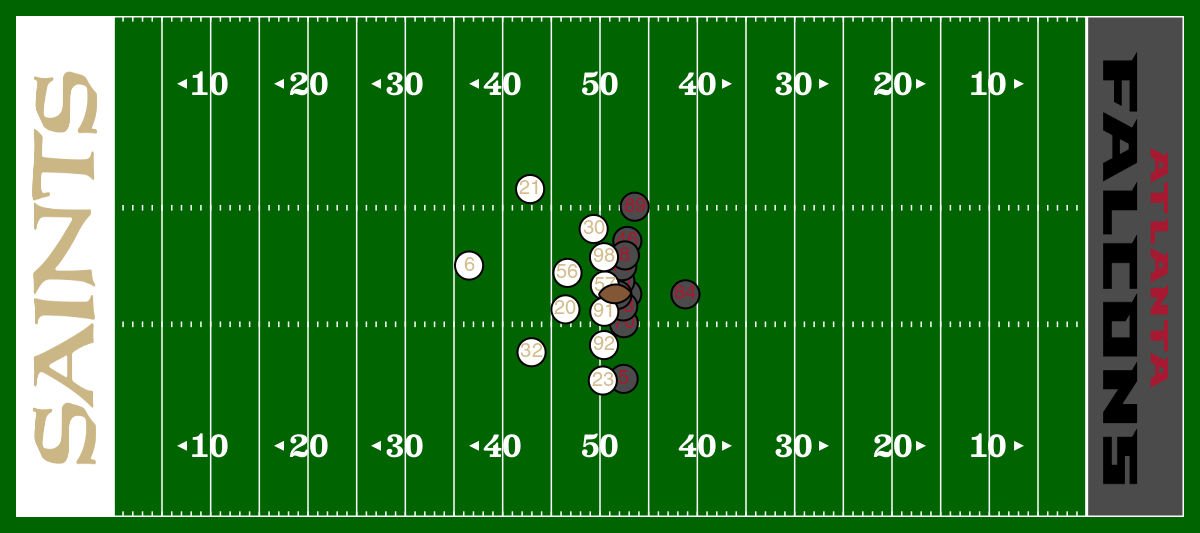
Decorating the Field
Next step – those end-zones are looking awful empty. Let’s try filling them up with some wordmarks, courtesy of the kind folks at the {nflverse} (I hear they’re a great bunch, very handsome, that John Edwards fella in particular).
We’ll first figure out who the team with the ball is on the play, then figure out which direction the play is going offensively – left to right. From there, we’ll plot the wordmark of the defensive team in the end-zone in the direction of the play, and the possession team in the opposite end-zone. Let’s pull in the plays.csv file and join it to figure out which team has the ball. We can then read in wordmarks for the possessing and defensive teams:
plays = CSV.read("data/plays.csv",DataFrame)
pos_team = plays[:,[:gameId, :playId, :possessionTeam, :defensiveTeam, :yardlineSide, :yardlineNumber, :yardsToGo]]
frame = innerjoin(frame,pos_team,on = [:gameId, :playId])
using Images
wordmark_pos = load("visuals/" * frame.possessionTeam[1] * "-wordmark.png")
wordmark_def = load("visuals/" * frame.defensiveTeam[1] * "-wordmark.png")

That wordmark is looking good! Next step – we’ll figure out the play direction, and based on that, plot the wordmarks (along with the team colors) in the correct endzones.
f, = base_figure()
plot_field()
# plot the end-zones
# we do this first to make sure the end-zones are layered under the players!
if frame.playDirection[1] == "left"
    poly!(
        Rect(0,0,10,53.3),
        strokecolor = :white,
        strokewidth = 3,
        color = String(frame.color[frame.defensiveTeam .== frame.club][1])
    )
    poly!(
        Rect(110,0,10,53.3),
        strokecolor = :white,
        strokewidth = 3,
        color = String(frame.color[frame.possessionTeam .== frame.club][1])
    )
    image!(
        [120,110],[53,0],wordmark_pos
    )
    image!(
        [0,10],[0,53],wordmark_def
    )
else
    poly!(
        Rect(0,0,10,53.3),
        strokecolor = :white,
        strokewidth = 3,
        color = String(frame.color[frame.possessionTeam .== frame.club][1])
    )
    poly!(
        Rect(110,0,10,53.3),
        strokecolor = :white,
        strokewidth = 3,
        color = String(frame.color[frame.defensiveTeam .== frame.club][1])
    )
    image!(
        [120,110],[53,0],wordmark_def
    )
    image!(
        [0,10],[0,53],wordmark_pos
    )
end
# okay, now we can plot the players
plot_players(frame)
f
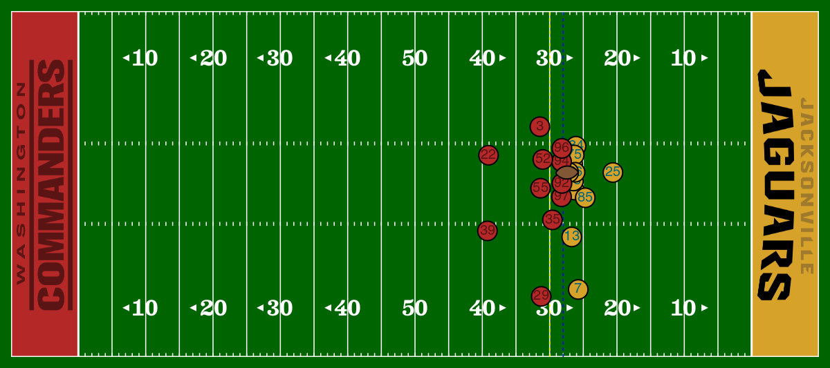
Oh helllllllll yeah. Alright, we’re missing one more thing. We want this to look at least a little like what it does on TV, so to make things clearer, we’re going to use the play data and plot the line of scrimmage in blue and the line to gain in yellow. We’ll wrap this into the same logic that determines which way to place the end-zones (and which way the ball is going):
f, = base_figure()
plot_field()
yardline_100 = ifelse(frame.yardlineSide[1] == frame.possessionTeam[1],50 - (50 - frame.yardlineNumber[1]), 50 + (50 - frame.yardlineNumber[1]))
if frame.playDirection[1] == "left"
    poly!(
        Rect(0,0,10,53.3),
        strokecolor = :white,
        strokewidth = 3,
        color = String(frame.color[frame.defensiveTeam .== frame.club][1])
    )
    poly!(
        Rect(110,0,10,53.3),
        strokecolor = :white,
        strokewidth = 3,
        color = String(frame.color[frame.possessionTeam .== frame.club][1])
    )
    image!(
        [120,110],[53,0],wordmark_pos
    )
    image!(
        [0,10],[0,53],wordmark_def
    )
    # line of scrimmage in blue, dashed
    vlines!(
        110 - yardline_100,
        color = :blue,
        linestyle = :dash
    )
    # line to gain -- in yellow, of course
    vlines!(
        110 - yardline_100 - frame.yardsToGo[1],
        color = :yellow,
        linestyle = :dash
    )
else
    poly!(
        Rect(0,0,10,53.3),
        strokecolor = :white,
        strokewidth = 3,
        color = String(frame.color[frame.possessionTeam .== frame.club][1])
    )
    poly!(
        Rect(110,0,10,53.3),
        strokecolor = :white,
        strokewidth = 3,
        color = String(frame.color[frame.defensiveTeam .== frame.club][1])
    )
    image!(
        [120,110],[53,0],wordmark_def
    )
    image!(
        [0,10],[0,53],wordmark_pos
    )
    vlines!(
        10 + yardline_100,
        color = :blue,
        linestyle = :dash
    )
    vlines!(
        10 + yardline_100 + frame.yardsToGo[1],
        color = :yellow,
        linestyle = :dash
    )
end
plot_players(frame)
f

Putting it all together
Terrific, looks like our field is ready to go. Like the other parts of the plot, let’s wrap it in a function.
function plot_ez_and_lines(frame)
    wordmark_pos = load("visuals/" * frame.possessionTeam[1] * "-wordmark.png")
    wordmark_def = load("visuals/" * frame.defensiveTeam[1] * "-wordmark.png")
    yardline_100 = ifelse(frame.yardlineSide[1] == frame.possessionTeam[1],50 - (50 - frame.yardlineNumber[1]), 50 + (50 - frame.yardlineNumber[1]))
    if frame.playDirection[1] == "left"

        poly!(
            Rect(0,0,10,53.3),
            strokecolor = :white,
            strokewidth = 3,
            color = String(frame.color[frame.defensiveTeam .== frame.club][1])
        )
        poly!(
            Rect(110,0,10,53.3),
            strokecolor = :white,
            strokewidth = 3,
            color = String(frame.color[frame.possessionTeam .== frame.club][1])
        )
        image!(
            [120,110],[53,0],wordmark_pos
        )
        image!(
            [0,10],[0,53],wordmark_def
        )
        vlines!(
            110 - yardline_100,
            color = :blue,
            linestyle = :dash
        )
        vlines!(
            110 - yardline_100 - frame.yardsToGo[1],
            color = :yellow,
            linestyle = :dash
        )
    else
        poly!(
            Rect(0,0,10,53.3),
            strokecolor = :white,
            strokewidth = 3,
            color = String(frame.color[frame.possessionTeam .== frame.club][1])
        )
        poly!(
            Rect(110,0,10,53.3),
            strokecolor = :white,
            strokewidth = 3,
            color = String(frame.color[frame.defensiveTeam .== frame.club][1])
        )
        image!(
            [120,110],[53,0],wordmark_def
        )
        image!(
            [0,10],[0,53],wordmark_pos
        )
        vlines!(
            10 + yardline_100,
            color = :blue,
            linestyle = :dash
        )
        vlines!(
            10 + yardline_100 + frame.yardsToGo[1],
            color = :yellow,
            linestyle = :dash
        )
    end
end
plot_ez_and_lines (generic function with 1 method)
Now with just a couple of lines, we can plot any frame from any play:
new_frame = week1[(week1.gameId .== 2022091109) .& (week1.playId .== 2404) .& (week1.frameId .== 5),:]
new_frame = innerjoin(new_frame,team_colors,on = :club => :team)
new_frame = innerjoin(new_frame,home_away,on = :gameId)
new_frame.color = ifelse.(new_frame.homeTeamAbbr .== new_frame.club, new_frame.dark, new_frame.light)
new_frame = innerjoin(new_frame,pos_team,on = [:gameId, :playId])
f, = base_figure()
plot_field()
plot_ez_and_lines(new_frame)
plot_players(new_frame)
f
We’ll want the ability to functionalize this further, to make it easier to plot the frames of individual plays. To do this, let’s prepare a DataFrame with all of the information we’ll need to plot plays, and turn it into a function to load it into memory.
function plot_df(weeks = 1:9, data_dir = "data")
    # read in data
    plays = CSV.read(data_dir * "/plays.csv",DataFrame)
    team_colors = CSV.read(download("https://gist.githubusercontent.com/john-b-edwards/7197daa7128088f2cb5bddef4e09bfa7/raw/8af4fb83609104fa14950cde5cc31d4d95a247b9/nfl_colors.csv"), DataFrame)
    games = CSV.read(data_dir * "/games.csv",DataFrame)
    home_away = games[:,[:gameId, :homeTeamAbbr]]
    dfs = [CSV.read(data_dir * "/tracking_week_" * string(week) * ".csv",DataFrame) for week in weeks]
    df = vcat(dfs...)
    df = innerjoin(df,team_colors,on = :club => :team)
    df = innerjoin(df,home_away,on = :gameId)
    df.color = ifelse.(df.homeTeamAbbr .== df.club, df.dark, df.light)
    df = innerjoin(df,pos_team,on = [:gameId, :playId])
    return(df)
end
main_df = plot_df()
| Row | gameId | playId | nflId | displayName | frameId | time | jerseyNumber | club | playDirection | x | y | s | a | dis | o | dir | event | dark | light | text | homeTeamAbbr | color | possessionTeam | defensiveTeam | yardlineSide | yardlineNumber | yardsToGo |
|---|---|---|---|---|---|---|---|---|---|---|---|---|---|---|---|---|---|---|---|---|---|---|---|---|---|---|---|
| Int64 | Int64 | String7 | String31 | Int64 | String31 | String3 | String15 | String7 | Float64 | Float64 | Float64 | Float64 | Float64 | String7 | String31 | String31 | String7 | String7 | String7 | String3 | String7 | String3 | String3 | String3 | Int64 | Int64 | |
| 1 | 2022090800 | 56 | 35472 | Rodger Saffold | 1 | 2022-09-08 20:24:05.200000 | 76 | BUF | left | 88.37 | 27.27 | 1.62 | 1.15 | 0.16 | 231.74 | 147.9 | NA | #C60C30 | #ffffff | #00338D | LA | #ffffff | BUF | LA | BUF | 25 | 10 |
| 2 | 2022090800 | 56 | 35472 | Rodger Saffold | 2 | 2022-09-08 20:24:05.299999 | 76 | BUF | left | 88.47 | 27.13 | 1.67 | 0.61 | 0.17 | 230.98 | 148.53 | pass_arrived | #C60C30 | #ffffff | #00338D | LA | #ffffff | BUF | LA | BUF | 25 | 10 |
| 3 | 2022090800 | 56 | 35472 | Rodger Saffold | 3 | 2022-09-08 20:24:05.400000 | 76 | BUF | left | 88.56 | 27.01 | 1.57 | 0.49 | 0.15 | 230.98 | 147.05 | NA | #C60C30 | #ffffff | #00338D | LA | #ffffff | BUF | LA | BUF | 25 | 10 |
| 4 | 2022090800 | 56 | 35472 | Rodger Saffold | 4 | 2022-09-08 20:24:05.500000 | 76 | BUF | left | 88.64 | 26.9 | 1.44 | 0.89 | 0.14 | 232.38 | 145.42 | NA | #C60C30 | #ffffff | #00338D | LA | #ffffff | BUF | LA | BUF | 25 | 10 |
| 5 | 2022090800 | 56 | 35472 | Rodger Saffold | 5 | 2022-09-08 20:24:05.599999 | 76 | BUF | left | 88.72 | 26.8 | 1.29 | 1.24 | 0.13 | 233.36 | 141.95 | NA | #C60C30 | #ffffff | #00338D | LA | #ffffff | BUF | LA | BUF | 25 | 10 |
| 6 | 2022090800 | 56 | 35472 | Rodger Saffold | 6 | 2022-09-08 20:24:05.700000 | 76 | BUF | left | 88.8 | 26.7 | 1.15 | 1.42 | 0.12 | 234.48 | 139.41 | pass_outcome_caught | #C60C30 | #ffffff | #00338D | LA | #ffffff | BUF | LA | BUF | 25 | 10 |
| 7 | 2022090800 | 56 | 35472 | Rodger Saffold | 7 | 2022-09-08 20:24:05.799999 | 76 | BUF | left | 88.87 | 26.64 | 0.93 | 1.69 | 0.09 | 235.77 | 134.32 | NA | #C60C30 | #ffffff | #00338D | LA | #ffffff | BUF | LA | BUF | 25 | 10 |
| 8 | 2022090800 | 56 | 35472 | Rodger Saffold | 8 | 2022-09-08 20:24:05.900000 | 76 | BUF | left | 88.91 | 26.59 | 0.68 | 1.74 | 0.07 | 240 | 131.01 | NA | #C60C30 | #ffffff | #00338D | LA | #ffffff | BUF | LA | BUF | 25 | 10 |
| 9 | 2022090800 | 56 | 35472 | Rodger Saffold | 9 | 2022-09-08 20:24:06.000000 | 76 | BUF | left | 88.94 | 26.57 | 0.42 | 1.74 | 0.04 | 243.56 | 122.29 | NA | #C60C30 | #ffffff | #00338D | LA | #ffffff | BUF | LA | BUF | 25 | 10 |
| 10 | 2022090800 | 56 | 35472 | Rodger Saffold | 10 | 2022-09-08 20:24:06.099999 | 76 | BUF | left | 88.95 | 26.58 | 0.14 | 1.83 | 0.01 | 246.07 | 85.87 | NA | #C60C30 | #ffffff | #00338D | LA | #ffffff | BUF | LA | BUF | 25 | 10 |
| 11 | 2022090800 | 56 | 35472 | Rodger Saffold | 11 | 2022-09-08 20:24:06.200000 | 76 | BUF | left | 88.92 | 26.6 | 0.26 | 1.9 | 0.03 | 252.65 | 326.63 | NA | #C60C30 | #ffffff | #00338D | LA | #ffffff | BUF | LA | BUF | 25 | 10 |
| 12 | 2022090800 | 56 | 35472 | Rodger Saffold | 12 | 2022-09-08 20:24:06.299999 | 76 | BUF | left | 88.9 | 26.63 | 0.51 | 2.45 | 0.04 | 257.66 | 315.55 | NA | #C60C30 | #ffffff | #00338D | LA | #ffffff | BUF | LA | BUF | 25 | 10 |
| 13 | 2022090800 | 56 | 35472 | Rodger Saffold | 13 | 2022-09-08 20:24:06.400000 | 76 | BUF | left | 88.84 | 26.68 | 0.81 | 2.03 | 0.08 | 262.09 | 311.72 | NA | #C60C30 | #ffffff | #00338D | LA | #ffffff | BUF | LA | BUF | 25 | 10 |
| ⋮ | ⋮ | ⋮ | ⋮ | ⋮ | ⋮ | ⋮ | ⋮ | ⋮ | ⋮ | ⋮ | ⋮ | ⋮ | ⋮ | ⋮ | ⋮ | ⋮ | ⋮ | ⋮ | ⋮ | ⋮ | ⋮ | ⋮ | ⋮ | ⋮ | ⋮ | ⋮ | ⋮ |
| 12187387 | 2022110700 | 3787 | NA | football | 33 | 2022-11-07 23:06:48.500000 | NA | football | right | 24.68 | 20.48 | 3.76 | 5.15 | 0.47 | NA | NA | NA | #825736 | #825736 | #825736 | NO | #825736 | NO | BAL | NO | 11 | 10 |
| 12187388 | 2022110700 | 3787 | NA | football | 34 | 2022-11-07 23:06:48.599999 | NA | football | right | 25.0 | 20.33 | 3.34 | 4.0 | 0.36 | NA | NA | NA | #825736 | #825736 | #825736 | NO | #825736 | NO | BAL | NO | 11 | 10 |
| 12187389 | 2022110700 | 3787 | NA | football | 35 | 2022-11-07 23:06:48.700000 | NA | football | right | 25.29 | 20.2 | 2.99 | 3.17 | 0.31 | NA | NA | NA | #825736 | #825736 | #825736 | NO | #825736 | NO | BAL | NO | 11 | 10 |
| 12187390 | 2022110700 | 3787 | NA | football | 36 | 2022-11-07 23:06:48.799999 | NA | football | right | 25.54 | 20.07 | 2.72 | 2.7 | 0.29 | NA | NA | NA | #825736 | #825736 | #825736 | NO | #825736 | NO | BAL | NO | 11 | 10 |
| 12187391 | 2022110700 | 3787 | NA | football | 37 | 2022-11-07 23:06:48.900000 | NA | football | right | 25.76 | 19.93 | 2.49 | 2.37 | 0.26 | NA | NA | NA | #825736 | #825736 | #825736 | NO | #825736 | NO | BAL | NO | 11 | 10 |
| 12187392 | 2022110700 | 3787 | NA | football | 38 | 2022-11-07 23:06:49.000000 | NA | football | right | 25.95 | 19.85 | 2.06 | 2.56 | 0.2 | NA | NA | NA | #825736 | #825736 | #825736 | NO | #825736 | NO | BAL | NO | 11 | 10 |
| 12187393 | 2022110700 | 3787 | NA | football | 39 | 2022-11-07 23:06:49.099999 | NA | football | right | 26.1 | 19.76 | 1.69 | 2.6 | 0.17 | NA | NA | NA | #825736 | #825736 | #825736 | NO | #825736 | NO | BAL | NO | 11 | 10 |
| 12187394 | 2022110700 | 3787 | NA | football | 40 | 2022-11-07 23:06:49.200000 | NA | football | right | 26.22 | 19.68 | 1.37 | 2.58 | 0.15 | NA | NA | tackle | #825736 | #825736 | #825736 | NO | #825736 | NO | BAL | NO | 11 | 10 |
| 12187395 | 2022110700 | 3787 | NA | football | 41 | 2022-11-07 23:06:49.299999 | NA | football | right | 26.32 | 19.61 | 1.07 | 2.74 | 0.12 | NA | NA | NA | #825736 | #825736 | #825736 | NO | #825736 | NO | BAL | NO | 11 | 10 |
| 12187396 | 2022110700 | 3787 | NA | football | 42 | 2022-11-07 23:06:49.400000 | NA | football | right | 26.39 | 19.56 | 0.8 | 2.49 | 0.09 | NA | NA | NA | #825736 | #825736 | #825736 | NO | #825736 | NO | BAL | NO | 11 | 10 |
| 12187397 | 2022110700 | 3787 | NA | football | 43 | 2022-11-07 23:06:49.500000 | NA | football | right | 26.45 | 19.52 | 0.57 | 2.38 | 0.07 | NA | NA | NA | #825736 | #825736 | #825736 | NO | #825736 | NO | BAL | NO | 11 | 10 |
| 12187398 | 2022110700 | 3787 | NA | football | 44 | 2022-11-07 23:06:49.599999 | NA | football | right | 26.49 | 19.5 | 0.35 | 2.13 | 0.05 | NA | NA | NA | #825736 | #825736 | #825736 | NO | #825736 | NO | BAL | NO | 11 | 10 |
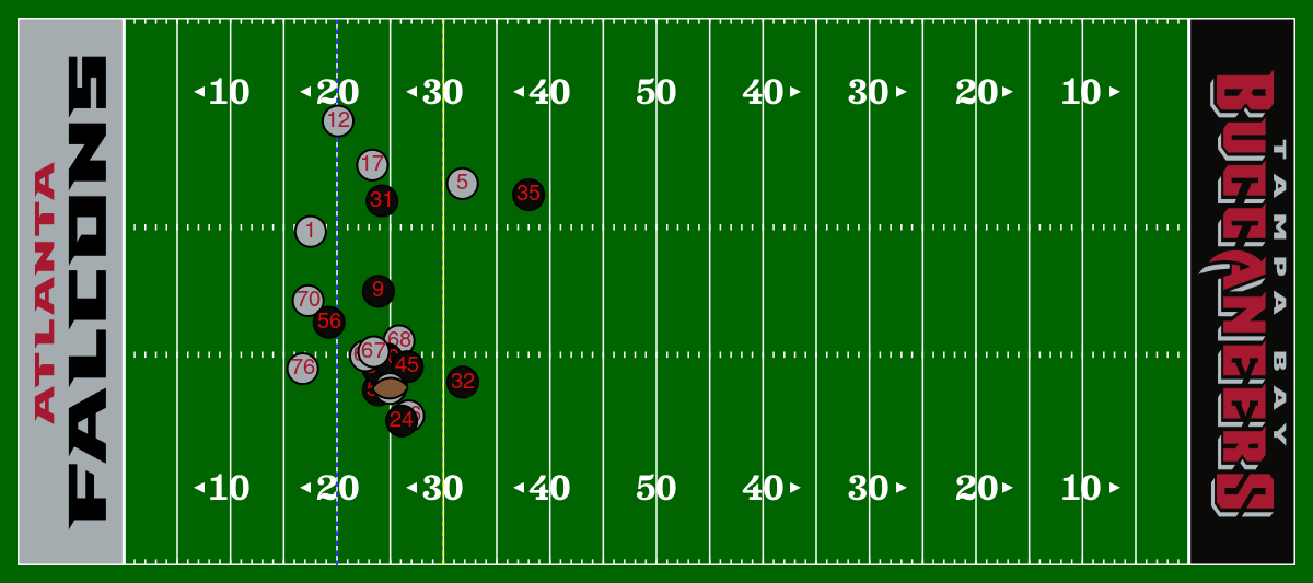
Now, we can make a function to just plot any frame of any play we query.
function plot_frame(df, gameId, playId, frameId)
    f, = base_figure()
    plot_field()
    frame = df[(df.gameId .== gameId) .& (df.playId .== playId) .& (df.frameId .== frameId),:]
    plot_ez_and_lines(frame)
    plot_players(frame)
    return(f)
end
plot_frame(main_df, 2022100908, 210, 40)
So we can now plot any frame from any play. How do we coalesce this into an animation of the play? Makie allows us to make a Gif of a play super easily, with the record() function. We’ll simply filter down to a specific play, then iterate over all the frames of the play and record each plot, then string those together to create a play animation.
function animate_play(df, gameId, playId)
    frames = 1:maximum(df.frameId[(df.gameId .== gameId) .& (df.playId .== playId)])
    # we buffer the animation with some still frames to make looping a little less jumpy
    frames = [repeat([1],5);frames;repeat([maximum(df.frameId[(df.gameId .== gameId) .& (df.playId .== playId)])],5)]
    f, ax = base_figure()
    record(f, "play.gif", frames; framerate = 15) do frame
        empty!(ax)
        plot_field()
        plot_ez_and_lines(df[(df.gameId .== gameId) .& (df.playId .== playId) .& (df.frameId .== frame),:])
        plot_players(df[(df.gameId .== gameId) .& (df.playId .== playId) .& (df.frameId .== frame),:])
    end
end
animate_play(main_df, 2022100908, 210)
"play.gif"
Extensions
I’m going to put a bow on this notebook here – however, there are a ton of additional extensions others can pursue with the logic laid out in this notebook. Makie is remarkably flexible and allows for a ton of customization, and Julia as a language provides a ton of opportunities for BDB work. Some examples of potential ways to extend this work:
- You can plot player velocity and/or acceleration using arrows
- You can plot the paths of individual players Family Circus style on a play
- You can create Voronoi Diagrams of field control on plays
- You can visualize the optimal path for a ball carrier on a play
I hope you found this notebook helpful, and I hope this sparked some interest in the wonderful language of Julia! Happy tackling!